A supervised ADMIXTURE run, assumes
that certain populations within a given dataset are 100% of a
certain ancestry, so for instance, given one wants to run ADMIXTURE at
K=10 in supervised mode, then 10 different populations that are
assumed to come from the 10 putative ancestral clusters that the software will infer, or rather will be forced to infer, must be manually selected.
I wanted to explore this type of a run
on a global basis and purposefully select populations that not only may form their own
clusters in an unsupervised run, but are also thought to be within
the 'trunk', bifurcation 'nodes' and end 'branches' of the ancestral 'tree' of all people.
The basis of this run is the global
dataset than can be downloaded in PLINK format from here. The
dataset, a superset of the African dataset that I have been thus far utilizing,
contains 3,970 individuals from around the world typed at 27,022 genome-wide SNPs.
A 3 dimensional, as well as a dim1 vs
dim2, MDS plot labelled according to the median coordinates of the population
groups for this dataset can be seen below:


The general structure of a globally
spread PCA/MDS plot is well known and understood, the first principal
component, describing the highest variation of all the components,
separates Africans from non-Africans, while the second principal
component separates West Asians/Europeans from East Asians, Oceanians
and Native Americans. The 3rd principal component can be
however shaky, in the plot above it separates Native Americans from
the rest, however other sources have shown that the 3rd
principal component in a global PCA separates divergent hunter
gatherers (like the Hadza, Sandawe, San and Pygmies) from every body
else, perhaps a 3-D PCA generated from full genome scans will put this
to rest once and for all.
Selection of Populations for
Supervision
To select the 10 populations
appropriate for supervision, I first resorted to an unsupervised K=14 run of this same global dataset that I had carried out in the past, I did this in order
to get a rough idea of where the cluster peaks in general for this
global (albeit very west Eurasian heavy) dataset were. The top five
cluster peaking populations for the k=14 unsupervised run can be seen
below:
Cluster1:
iban,singapore-malay,cambodian,thai,khmer-cambodian
Cluster2:
lithuanians,orcadian,belorussian,utahn-whites,basque
Cluster3:
irula,tn-dalit,malayan,ap-mala,ap-madiga
Cluster4:
dogon,yoruba,bambaran,igbo,brong
Cluster5:
east-greenlanders,west-greenlanders,chukchis,koryaks,pima
Cluster6:
pygmy,mbutipygmy,biakapygmy,alur,fang
Cluster7:
nganassans,evenkis,yakut,dolgans,buryats
Cluster8:
kalash,urkarah,lezgins,brahui,georgians
Cluster9:
tunisia,yemen-jews,sahara-occ,saudis,bedouin
Cluster10:
japanese,she,chinese-americans,chinese,beijing-chinese
Cluster11:
karitiana,surui,colombian,totonac,pima
Cluster12:
maasai,hadza,EtO,EtJ,bulala
Cluster13:
papuan,melanesian,tongan,samoan,paniya
Cluster14:
san-nb,!kung,san,sotho/tswana,xhosa
As mentioned before, since I selected
to do a supervised ADMIXTURE run at K=10, I picked 10 of the
clusters, or rather the peaking populations of those clusters, out of
the 14 total, based on various criteria including absolute cluster
peaks, isolated populations, divergent populations, populations found
at crucial nodes and endpoints of the OOA migration, and so forth,
the populations I selected are seen highlighted in yellow above,
and where they generally come from are highlighted in the map below.

A lot of putative maps for the OOA
migration routes are also available online, most of them are just
rough guides and miss some of the finer points, but are generally
good for an overview of the OOA and subsequent human migration
routes, the below is one such map for reference;

Filtering the Supervised ADMIXTURE
run.
Based on the 10 populations selected, I
run ADMIXTURE in the supervised mode, on a technical note, to run
ADMIXTURE in such a mode a *.pop file needs to be first created and
placed in the same folder as where the common files (.bed/.bim/.fam
files) are placed, see the instructions of the software for details.
The K10 supervised ADMIXTURE median cluster frequency results, as
well as the standard deviation of each cluster for the 172 uniquely
entered population groups can be downloaded here.
However, since I wanted to reduce the
standard deviations of the clusters by removing outliers , I
performed a studentize > 2 computation on each cluster found per
sample within each population group, 1238 such individual samples
failed the test of having a studentize value < 2, so I proceeded
to rerun the K10 ADMIXTURE utility in supervised mode again with
those samples removed. The filtration of the samples using the above
procedure thus left me with 2,732 samples typed at 27,022 SNPs.
Results.
The median matrix for the proportions
of the clusters, as well as the standard deviations for the second
and final iteration can be downloaded here. It is worthwhile to note
that the filtration of the samples had an impact on the sample
standard deviations of each cluster per population group, before
filtration, there was a total count of 124 sample standard deviation
elements that had values > 5%, after filtration that frequency
dropped to 60 or to slightly less than a half.
Some of the Clusters were more
numerously represented in different groups and geographical areas
than others, highlighting the sample bias inherent in the dataset, I
have therefore arranged the graphical representation of the results from highest representation of a certain cluster in the dataset (for populations showing >5% cluster
representation), to those less numerously represented.
- The Basque Cluster.This cluster had the most numerous representation in the dataset, concentrated most in West Asia and Europe, 90 population groups in the dataset carried it at frequency greater than 5%.

- The Irula Cluster.The next cluster to have the highest representation, and mostly prevalent in South and Central Asia, this cluster was found at >5% in 60 population groups of the Dataset.

- The Ethiopian Cluster.This cluster had it's highest representation in East and North Africa, as well as the Arabian Peninsula, it was mostly represented by 49 population groups in the dataset, whom had a frequency of it >5%.

- The Japanese Cluster.This cluster had a representation of >5% in 48 population groups of the Dataset, with high prevalence in East and south east Asia.

- The Nganassan Cluster.This North Asian based cluster was best represented by 36 populations in the Dataset, it was prevalent as far South as with Central Asians.

- The Dogon Cluster.A cluster based in West Africa, was represented by 32 populations at >5%, present in East, Central and South Africa and tapering off in Northern Africa.

- The Mbuti Pygmy Cluster.With lower representation in this dataset, but clearly unique, the Mbuti Pygmy cluster was present in only 14 populations @ >5%, its widest distribution is in Central Africa, but can also be found in Eastern Africa.

- The Karitiana Cluster.Represented with only 13 populations in the dataset, essentially Native American specific, however the cluster was also present in North Asian populations like the Chukchis and Greenlanders.

- The San Cluster.One of the least represented and most unique clusters, this Khoisan specific cluster was only present in 12 of the sampled groups in a relatively significant amount, other hunter gatherers also seem to carry this cluster in appreciable frequencies along with some Bantu South Africans.
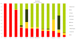
- The Papuan Cluster.The least represented cluster, due to small amounts of Oceanian and Oceanian-like groups of samples, this cluster was only represented at >5% in only 8 groups. South East Asians and others that carried the Japanese cluster in significant amounts, also carry the Papuan cluster.
 The Fst distances for the 10 clusters can be seen below.


-This is data only from ~27,000 SNPs, the average variation between two human beings is said to be ~3 million SNPs, therefore it would be hard to say what results another set of 27,000 SNPs from a different location or set of locations in the genome may reveal if this exact same analysis was run, however on the other hand, the general structure of human genetic variation on a global level, for instance as revealed by PCA, is said to be pretty robust even at 1,000 SNPs.
-A better globally represented dataset with less gaps allowing for more continuity between populations could also yield different results.


''The 3rd principal component can be however shaky, in the plot above it separates Native Americans from the rest, however other sources have shown that the 3rd principal component in a global PCA separates divergent hunter gatherers (like the Hadza, Sandawe, San and Pygmies) from every body else, perhaps a 3-D PCA generated from full genome scans will put this to rest once and for all.''
ReplyDeleteThis can be affected by sample size. Tishkoff had more HG samples and less East Asians.
Then how come complete genome sequences of the san show more nucleotide substitution differences with each other than the differences observed between a European and an East Asian?
DeleteThere are now San based SNP panels available. Perhaps you can check whether it has any significant effect on the 3rd principal component relative to a European or Asian based SNP panel.
Deleteftp://ftp.cephb.fr/hgdp_supp10/
Not a lot of change with those HGDP samples ascertained for the SAN, see here , C3 still separates the Native Americans from the rest, there is a slight shift of the SAN on C3 (in the opposite direction of the Native Americans) but the majority of the shift is with the NA, still, we are only talking ~163K SNPs versus the entire genome.
DeleteI still think it's mainly a sample size issue, because of the low amount of San samples, if a lot more are added it most likely will show different things.
Delete